Examples¶

Constant current charge constant voltage discharge¶

This is based on [Journal of The Electrochemical Society, 152 (5) D79-D87 (2005)] by M. Verbrugge and P. Liu. It illustrates how easy it is to specify complex operating conditions for energy storage devices in pycap.

from pycap import EnergyStorageDevice,PropertyTree
from pycap import initialize_data,report_data,plot_data
from matplotlib import pyplot
%matplotlib inline

The supercapacitor is initially fully discharged. It is charged to $1.7\ \mathrm{V}$ at a constant current of $100\ \mathrm{A}$ . Subsequently, a constant $1.4\ \mathrm{V}$ is applied for $5\ \mathrm{s}$ and the supercapacitor is allowed to rest at open circuit potential for $3\ \mathrm{min}$ . This sequence is repeated for a series of charge potentials at $0.1\ \mathrm{V}$ increments from $1.8$ to $2.4\ \mathrm{V}$ . The routine defined below, run_verbrugge_experiment, implements that experiment and records measurements for the time, current and voltage.

def run_verbrugge_experiment(device):
    charge_current=1.65e-3 # ampere
    discharge_voltage=1.4 # volt
    discharge_time=5.0 # second
    rest_time=180.0 # second
    time_step=0.1 # second
    time=0.0
    data=initialize_data()
    for charge_voltage in [1.7,1.8,1.9,2.0,2.1,2.2,2.3,2.4]:
        # constant current charge
        while device.get_voltage()<charge_voltage:
            time+=time_step
            device.evolve_one_time_step_constant_current(time_step,charge_current)
            report_data(data,time,device)
        # constant voltage discharge
        tick=time
        while time-tick<discharge_time:
            time+=time_step
            device.evolve_one_time_step_constant_voltage(time_step,discharge_voltage)
            report_data(data,time,device)
        # rest at open circuit
        tick=time
        while time-tick<rest_time:
            time+=time_step
            device.evolve_one_time_step_constant_current(time_step,0.0)
            report_data(data,time,device)
    return data

Make an energy storage device (here a supercapacitor) and run the experiment.

input_database=PropertyTree()
input_database.parse_xml('super_capacitor.xml')
# no faradaic processes
input_database.put_double('device.material_properties.electrode_material.exchange_current_density',0.0)
device=EnergyStorageDevice(input_database.get_child('device'))
# run experiment
data=run_verbrugge_experiment(device)

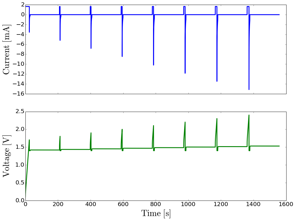
Postprocess the results.

time=data['time']
current=data['current']
voltage=data['voltage']
label_fontsize=30
tick_fontsize=20
labelx=-0.05
labely=0.5
plot_linewidth=3
f,axarr=pyplot.subplots(2,sharex=True,figsize=(16,12))
axarr[0].plot(time,1e+3*current,'b-',lw=plot_linewidth)
axarr[0].set_ylabel(r'$\mathrm{Current\ [mA]}$',fontsize=label_fontsize)
axarr[0].get_yaxis().set_tick_params(labelsize=tick_fontsize)
axarr[0].yaxis.set_label_coords(labelx,labely)
axarr[1].plot(time,voltage,'g-',lw=plot_linewidth)
axarr[1].set_ylabel(r'$\mathrm{Voltage\ [V]}$',fontsize=label_fontsize)
axarr[1].set_xlabel(r'$\mathrm{Time\ [s]}$',fontsize=label_fontsize)
axarr[1].get_yaxis().set_tick_params(labelsize=tick_fontsize)
axarr[1].get_xaxis().set_tick_params(labelsize=tick_fontsize)
axarr[1].yaxis.set_label_coords(labelx,labely)
pyplot.show()

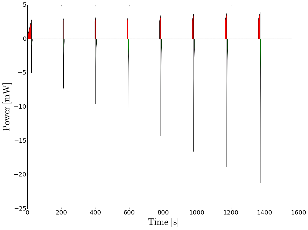
Plot the power versus time. The red surface area represents the energy used to charge the supercapacitor and the green on the power pulses is the energy recovered.

power=current*voltage
pyplot.figure(figsize=(16,12))
pyplot.fill_between(time,1e+3*power,0,where=power>0,facecolor='r')
pyplot.fill_between(time,1e+3*power,0,where=power<0,facecolor='g')
pyplot.xlabel(r'$\mathrm{Time\ [s]}$',fontsize=label_fontsize)
pyplot.ylabel(r'$\mathrm{Power\ [mW]}$',fontsize=label_fontsize)
pyplot.gca().get_xaxis().set_tick_params(labelsize=tick_fontsize)
pyplot.gca().get_yaxis().set_tick_params(labelsize=tick_fontsize)
pyplot.show()