Energy storage devices
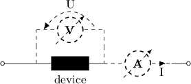
Only the electrical current  and voltage
  of the device are
measurable. Several operating conditions are possibles. One may want to
impose:
of the device are
measurable. Several operating conditions are possibles. One may want to
impose:
- The voltage
- The electrical current
- The load
the device is subject to.
- The power
.
The class pycap.EnergyStorageDevice is an abstract representation
for an energy storage device. It can evolve in time at various operating
conditions and return the voltage drop across itself and the electrical
current that flows through it.
The rest of this section describes the energy storage devices that are available in Cap, namely:
- Equivalent circuits
- Supercapacitors
Equivalent circuits
Series RC
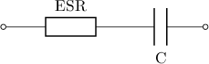
A resistor and a capacitor are connected in series (denoted  and
and  in the figure above).
type                SeriesRC
series_resistance     5.0e-3 ; [ohm]
capacitance           3.0    ; [fahrad]
Above is the database to build a  capacitor in series with a
 resistance.
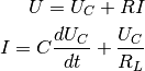
 stands for the voltage across the capacitor.
Its capacitance,
stands for the voltage across the capacitor.
Its capacitance,  , represents its ability to store electric charge.
The equivalent series resistance,
, represents its ability to store electric charge.
The equivalent series resistance,  , add a real component to the
impedance of the circuit:
, add a real component to the
impedance of the circuit:
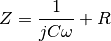
As the frequency goes to infinity, the capacitive impedance approaches zero
and becomes significant.
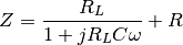
Parallel RC
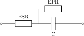
An extra resistance is placed in parallel of the capacitor. It can be instantiated by the following database.
type                 ParallelRC
parallel_resistance      2.5e+6 ; [ohm]
series_resistance       50.0e-3 ; [ohm]
capacitance              3.0    ; [fahrad]
type has been changed from SeriesRC to ParallelRC.
A  leakage resistance is specified.
 corresponds to the “leakage” resistance in parallel with the
capacitor. Low values of imply high leakage currents which means
the capacitor is not able to hold is charge.
The circuit complex impedance is given by:
corresponds to the “leakage” resistance in parallel with the
capacitor. Low values of imply high leakage currents which means
the capacitor is not able to hold is charge.
The circuit complex impedance is given by:
Supercapacitors
type is set to SuperCapacitor.
dim is used to select two- or three-dimensional simulations.
device {
    type SuperCapacitor
    dim 2
    geometry {
        [...]
    }
    material_properties {
        [...]
    }
}
Geometry
geometry {
    type supercapacitor

    anode_collector_thickness    5.0e-4 ; [centimeter]
    anode_electrode_thickness   50.0e-4 ; [centimeter]
    separator_thickness         25.0e-4 ; [centimeter]
    cathode_electrode_thickness 50.0e-4 ; [centimeter]
    cathode_collector_thickness  5.0e-4 ; [centimeter]
    geometric_area              25.0e-2 ; [square centimeter]
}
The thickness of each layer in the sandwich (anode collector, anode electrode, separator, cathode electrode, cathode current collector) can be adjusted independently from one another. The specified cross-sectional area applies to the whole stack.
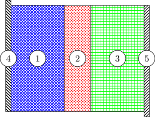
Schematic representation of the supercapacitor conventional sandwich-like configuration. 1: anode electrode, 2: separator, 3: cathode electrode, 4: anode collector, 5: cathode collector.
Governing equations
| collector | electrode | separator |
|---|---|---|
|
|
|


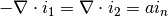

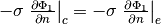
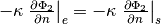
| collector-electrode interface | electrode-separator interface |
|---|---|
|
|
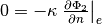
| boundary collector tab |
|---|
or
or
or
|

Ignoring the influence of the electrolyte concentration, the current density in the matrix and solution phases can be expressed by Ohm’s law as

 and
and  represent current density and potential; subscript
indices
represent current density and potential; subscript
indices  and
and  denote respectively the solid and the liquid
phases.
denote respectively the solid and the liquid
phases.  and
and  are the matrix and solution phase
conductivities.
are the matrix and solution phase
conductivities.
The total current density is given by  . Conservation of
charge dictates that
. Conservation of
charge dictates that

where  is the interfacial area per unit volume and the current
transferred from the matrix phase to the electrolyte
is the interfacial area per unit volume and the current
transferred from the matrix phase to the electrolyte  is the sum of
the double-layer the faradaic currents
is the sum of
the double-layer the faradaic currents
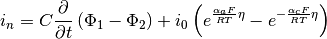
is the double-layer capacitance.  is the exchange current
density,
is the exchange current
density,  and
and  the anodic and cathodic charge
transfer coefficients, respectively.
the anodic and cathodic charge
transfer coefficients, respectively.  , , and
  stand
for Faraday’s constant, the universal gas constant and temperature.
stand
for Faraday’s constant, the universal gas constant and temperature.
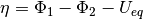
 is the overpotential relative to the equilibrium potential

Material properties
material_properties {
    anode {
        type           porous_electrode
        matrix_phase   electrode_material
        solution_phase electrolyte
    }
    cathode {
        type           porous_electrode
        matrix_phase   electrode_material
        solution_phase electrolyte
    }
    separator {
        type           permeable_membrane
        matrix_phase   separator_material
        solution_phase electrolyte
    }
    collector {
        type           current_collector
        metal_foil     collector_material
    }

    separator_material {
        void_volume_fraction             0.6       ;
        tortuosity_factor                1.29      ;
        pores_characteristic_dimension   1.5e-7    ; [centimeter]
        pores_geometry_factor            2.0       ;
        mass_density                     3.2       ; [gram per cubic centimeter]
        heat_capacity                    1.2528e3  ; [joule per kilogram kelvin]
        thermal_conductivity             0.0019e2  ; [watt per meter kelvin]
    }
    electrode_material {
        differential_capacitance         3.134     ; [microfarad per square centimeter]
        exchange_current_density         7.463e-10 ; [ampere per square centimeter]
        void_volume_fraction             0.67      ;
        tortuosity_factor                2.3       ;
        pores_characteristic_dimension   1.5e-7    ; [centimeter]
        pores_geometry_factor            2.0       ;
        mass_density                     2.3       ; [gram per cubic centimeter]
        electrical_resistivity           1.92      ; [ohm centimeter]
        heat_capacity                    0.93e3    ; [joule per kilogram kelvin]
        thermal_conductivity             0.0011e2  ; [watt per meter kelvin]
    }
    collector_material {
        mass_density                     2.7       ; [gram per cubic centimeter]
        electrical_resistivity          28.2e-7    ; [ohm centimeter]
        heat_capacity                    2.7e3     ; [joule per kilogram kelvin]
        thermal_conductivity           237.0       ; [watt per meter kelvin]
    }
    electrolyte {
        mass_density                     1.2       ; [gram per cubic centimeter]
        electrical_resistivity           1.49e3    ; [ohm centimeter]
        heat_capacity                    0.0       ; [joule per kilogram kelvin]
        thermal_conductivity             0.0       ; [watt per meter kelvin]
    }
}
The specific surface area per unit volume is estimated using

where  is the pore’s geometry factor (
 for
spheres, for cylinders, and
for
spheres, for cylinders, and  for slabs) and
  is
the pore’s characteristic dimension.
[M. W. Verbrugge and B. J. Koch, J. Electrochem. Soc., 150, A374 2003]
is
the pore’s characteristic dimension.
[M. W. Verbrugge and B. J. Koch, J. Electrochem. Soc., 150, A374 2003]
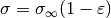
The solution electrical conductivity incorporates the effect
of porosity and tortuosity

where  is the liquid phase (free solution) conductivity,
 is the void volume fraction, and is the
tortuosity factor.
is the void volume fraction, and is the
tortuosity factor.
The solid phase conductivity is also corrected for porosity (and tortuosity???)
Batteries
NOT IMPLEMENTED