Electrochemical techniques¶

Cyclic charge discharge¶

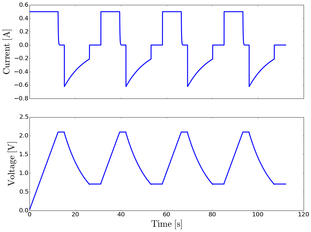
Cyclic Charge-Discharge is a common technique used to test the performance and cycle-life of energy storage devices. Most often, the charge and discharge are conducted at constant current until a set voltage is reached.

The following implements 4 cycles of a repetitive loop through several steps:

constant current charge at $0.5\ \mathrm{A}$ until voltage reaches a $2.1\ \mathrm{V}$ limit
potentiostatic hold until the current falls below $1\ \mathrm{mA}$ for a maximum duration time of $3\ \mathrm{min}$
rest at open circuit potential for $2\ \mathrm{s}$
constant load discharge at $3.33\ \mathrm{\Omega}$ to $0.7\ \mathrm{V}$
rest at open circuit potential for $5\ \mathrm{s}$

from pycap import PropertyTree,CyclicChargeDischarge,EnergyStorageDevice

# setup the experiment
ptree=PropertyTree()
ptree.put_string('start_with','charge')
ptree.put_int   ('cycles',4)
ptree.put_double('time_step',0.01)

ptree.put_string('charge_mode','constant_current')
ptree.put_double('charge_current',0.5)
ptree.put_string('charge_stop_at_1','voltage_greater_than')
ptree.put_double('charge_voltage_limit',2.1)
ptree.put_bool  ('charge_voltage_finish',True)
ptree.put_double('charge_voltage_finish_max_time',180)
ptree.put_double('charge_voltage_finish_current_limit',1e-3)
ptree.put_double('charge_rest_time',2)

ptree.put_string('discharge_mode','constant_load')
ptree.put_double('discharge_load',3.33)
ptree.put_string('discharge_stop_at_1','voltage_less_than')
ptree.put_double('discharge_voltage_limit',0.7)
ptree.put_double('discharge_rest_time',5)

ccd=CyclicChargeDischarge(ptree)

The property tree is populated interactively here but it can parse directly an input file. Please refer to other examples.

The CCD experiment can be started with a charge or a discharge step. The length of the test is defined by the cycle number and the loop end criteria.

The charge mode can be constant_current, constant_voltage, or constant_power. Two end criteria can be selected although only one is required. Note that they are no safeguards and poor end criteria will produce infinite loops! If voltage_finish is enabled (default value is False), the charge step proceeds to a potentiostatic step that ends after reaching the specified time voltage_finish_max_time or when the current falls between the limiting value voltage_finish_current_limit (absolute value). The voltage finish step makes little sense in case of a constant voltage charge and therefore is not allowed. The charge ends with an optional rest time period before proceeding with the next step.

The discharge process can be perfomed in four different modes: contant_current, contant_voltage, constant_power, or constant_load. End criteria must be chosen carfully here as well.

Let’s build an energy storage device, here a simple series RC circuit, with a $40\ \mathrm{m\Omega}$ resistor and a $3\ \mathrm{F}$ capacitor, and run the experiment.

# build an energy storage device
ptree=PropertyTree()
ptree.put_string('type','SeriesRC')
ptree.put_double('series_resistance',40e-3)
ptree.put_double('capacitance',3)
device=EnergyStorageDevice(ptree)

from pycap import initialize_data,plot_data

# run the experiment and visualize the measured data
data=initialize_data()
steps=ccd.run(device,data)

print "%d steps"%steps

%matplotlib inline
plot_data(data)

11213 time steps ( $\Delta t = 0.01\ \mathrm{s}$ ) are required to complete the CCD experiment. Below are plotted the measured current and voltage data versus time.

Cyclic voltammetry¶

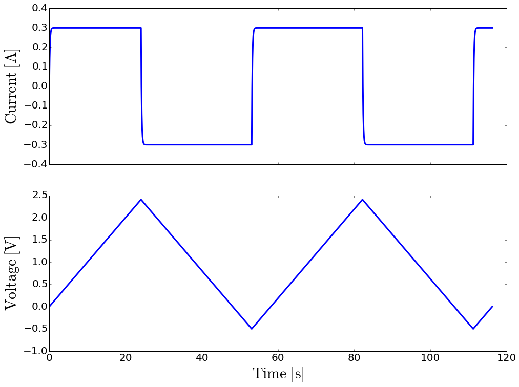
Cyclic Voltammetry (CV) is a widely-used electrochemical technique to investigate energy storage devices. It consists in measuring the current while varying linearly the voltage back and forth over a given range.

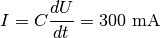
The voltage sweep applied to the device creates a current given by

$I = C \frac{dU}{dt}$

where $I$ is the current in ampere and $\frac{dU}{dt}$ is the scan rate of the voltage ramp.

The voltage scan rates for testing energy storage devices are usually between $0.1\ \mathrm{mV/s}$ and $\mathrm{1\ V/s}$ . Scan rates at the lower end of this range allow slow processes to occur; fast scans often show lower capacitance than slower scans and may produce large currents on high-value capacitors.

from pycap import PropertyTree, CyclicVoltammetry

# setup the experiment
ptree = PropertyTree()
ptree.put_double('initial_voltage', 0) # volt
ptree.put_double('final_voltage', 0) # volt
ptree.put_double('scan_limit_1', 2.4) # volt
ptree.put_double('scan_limit_2', -0.5) # volt
ptree.put_double('scan_rate', 100e-3) # volt per second
ptree.put_double('step_size', 5e-3) # volt
ptree.put_int('cycles', 2)
cv = CyclicVoltammetry(ptree)

Four parameters define the CV sweep range: The scan starts at initial_voltage, ramps to scan_limit_1, reverses and goes to scan_limit_2. Additional cycles start and end at scan_limit_2. The scan ends at final_voltage. Here, the sweep range is [ $2.4\ \mathrm{V}$ , $-0.5\ \mathrm{V}$ ]. It both starts and finishes at $0\ \mathrm{V}$ .

The rate of voltage change over time $\frac{dU}{dt}$ is specified using scan_rate which is here set to $100\ \mathrm{mV/s}$ . The linear ramp is imposed in increments of $5\ \mathrm{mV}$ . The number of sweep is controlled by cycles.

Here we run the experiment with a $3\ \mathrm{F}$ capacitor in series with a $50\ \mathrm{m\Omega}$ resistor.

# build an energy storage device
ptree=PropertyTree()
ptree.put_string('type','SeriesRC')
ptree.put_double('capacitance',3)
ptree.put_double('series_resistance',50e-3)
device=EnergyStorageDevice(ptree)

from pycap import initialize_data,report_data,plot_data
from pycap import plot_cyclic_voltammogram

# run the experiment and visualize the measured data
data=initialize_data()
steps=cv.run(device,data)

print "%d steps"%steps

%matplotlib inline
plot_data(data)
plot_cyclic_voltammogram(data)

2320 steps

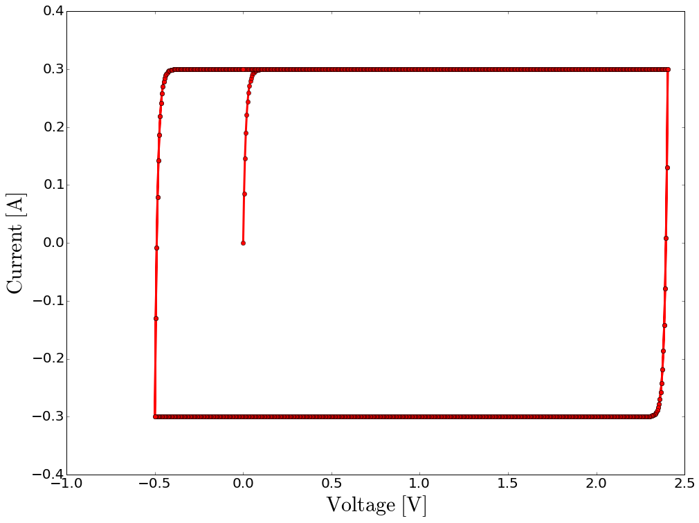
On the CV plot (current on the y-axis and voltage on the x-axis), we read

$I = C \frac{dU}{dt} = 300\ \mathrm{mA}$

as expected for a $3\ \mathrm{F}$ capacitor. For an ideal capacitor (i.e. no equivalent series resistance), the plot would be a perfect rectangle. The resistor causes the slow rise in the current at the scan’s start and rounds two corners of the rectangle. The time constant $\tau=RC$ controls rounding of corners.

Electrochemical impedance spectroscopy¶

Electrochemical Impedance Spectroscopy (EIS) is a powerful experimental method for characterizing electrochemical systems. This technique measures the complex impedance of the device over a range of frequencies.

A sinusoidal excitation signal (potential or current) is applied:

$E = E_0 + \sum_k E_k \sin (\omega_k t + \varphi_k)$

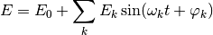
That signal consists in the superposition of AC sine waves with amplitude $E_k$ , angular frequency $\omega_k=2\pi kf$ , and phase shift $\phi_k$ . $E_0$ is the DC component.

; `eis.info` file

frequency_upper_limit  1e+3 ; hertz
frequency_lower_limit  1e-2 ; hertz
steps_per_decade          6

cycles                    2
ignore_cycles             1
steps_per_cycle         128

harmonics                 1
dc_voltage                0 ; volt
amplitudes             5e-3 ; volt
phases                    0 ; degree

In the input data above:

frequency_upper_limit, frequency_lower_limit, and steps_per_decade define the frequency range and the resolution on a log scale (for the fundamental frequency). Frequencies are scanned from the upper limit to the lower one.
Electric current and potential signals are sampled at regular time interval and steps_per_cycle controls the size of that interval. ignore_cycles allows to truncate the data in the Fourier analysis. It is best when (cycles - ignore_cycles) * steps_per_cycle is a power of two (most efficient in the discrete Fourier transform) but this does not have to be so.
harmonics allows to select what harmonics $k$ of the fundamental frequency $f$ to excite. amplitudes and phases are used to specify $E_k$ and $\varphi_k$ , respectively. They may be given as arrays and must have the same size. This multi-sine feature is experimental though. In principle, exciting simultaneously multiple frequencies reduces the computational cost associated with a full spectrum acquisition, but in practice, it is hard to maintain the quality of the data measurement without increasing the number of steps.

Below is an example of EIS measurement using Cap:

from pycap import PropertyTree, ElectrochemicalImpedanceSpectroscopy,\
                  NyquistPlot

# setup the experiment
ptree = PropertyTree()
ptree.parse.info('eis.info')
eis = ElectrochemicalImpedanceSpectroscopy(ptree)

# build an energy storage device and run the EIS measurement
eis.run(device)

# visualize the impedance spectrum
nyquist = NyquistPlot(filename='nyquist.png')
nyquist.update(eis)

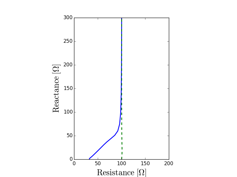
_images/nyquist_plot_no_faradaic_processes.png

On the Nyquist plot above, the solid blue line shows the impedance of a supercapacitor on the complex plane with the typical 45 degrees slope for the higher frequencies. The vertical dashed green line corresponds to an equivalent RC circuit.

Ragone plot¶

Conceptually, the y-axis describes how much energy is available and the the x-axis shows how quickly that energy can be delivered.